Neural Network Modeling of Ionospheric F2-Layer Electrodynamics

May 05, 2018 · past · ionosphere, machine learning, neural networks, space weather

• MSc Thesis (PDF)
• ANNIM-2D (JGR 2018)
• ANNIM-3D (JGR 2019)

This project developed one of the earliest neural-network–based ionospheric models capable of predicting global F2-layer peak density (NmF2) and peak height (hmF2) from long-term satellite and ground-based measurements. The work demonstrated that machine-learning approaches can replicate large-scale ionospheric electrodynamics traditionally captured only by empirical or physics-based models.

Context & Motivation

The high-latitude ionosphere is a dynamic plasma environment controlled by solar EUV radiation, geomagnetic forcing, and neutral wind circulation. Accurate estimates of NmF2 (peak electron density) and hmF2 (corresponding altitude) are essential for radio communication forecasting, satellite navigation accuracy, and space weather nowcasting.

Traditional ionospheric models fall into two camps:

• Physics-based models (e.g., TIEGCM, SAMI2/SAMI3) that solve continuity and momentum equations.
• Empirical models (e.g., IRI, NeQuick) that fit climatological data using analytical functions.

However, both approaches struggle with nonlinear responses to geomagnetic storms, solar minima, and Equatorial Ionization Anomaly. With the advent of large-scale radio occultation (RO) datasets from FORMOSAT-3/COSMIC, CHAMP, GRACE, and global Digisonde GIRO network, machine learning offered a viable alternative.

This project explored that possibility.

Approach / Methods

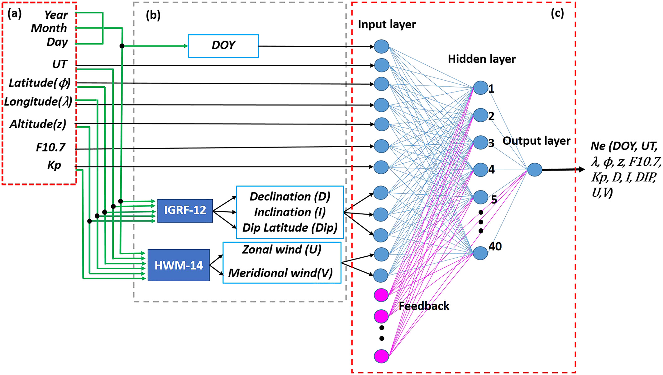
The core methodology was a feed-forward artificial neural network (ANN) trained to map observed and modeled ionospheric conditions, magnetic fields, solar activity, and winds to NmF₂ and hₘF₂.

Key elements:

• Input Data Sources

  • GPS-RO from COSMIC, CHAMP, GRACE
  • Digisonde GIRO network (confidence ≥ 90)
  • (Later extensions incorporated topside sounders – see ANNIM-3D)

• Architecture

  • Single hidden layer with 40 neurons
  • Levenberg–Marquardt backpropagation (fast convergence)
  • 70% training / 15% validation / 15% testing

• Two Training Paradigms (tested in thesis)

  • Single global network → underfit regional structures
  • Gridded neural networks → one ANN per 5° dip-lat × 15° longitude patch

• Physics-aware augmentation

  • Neutral zonal/meridional winds from HWM-14
  • IGRF magnetic field parameters (declination, inclination)

Key Results & Findings

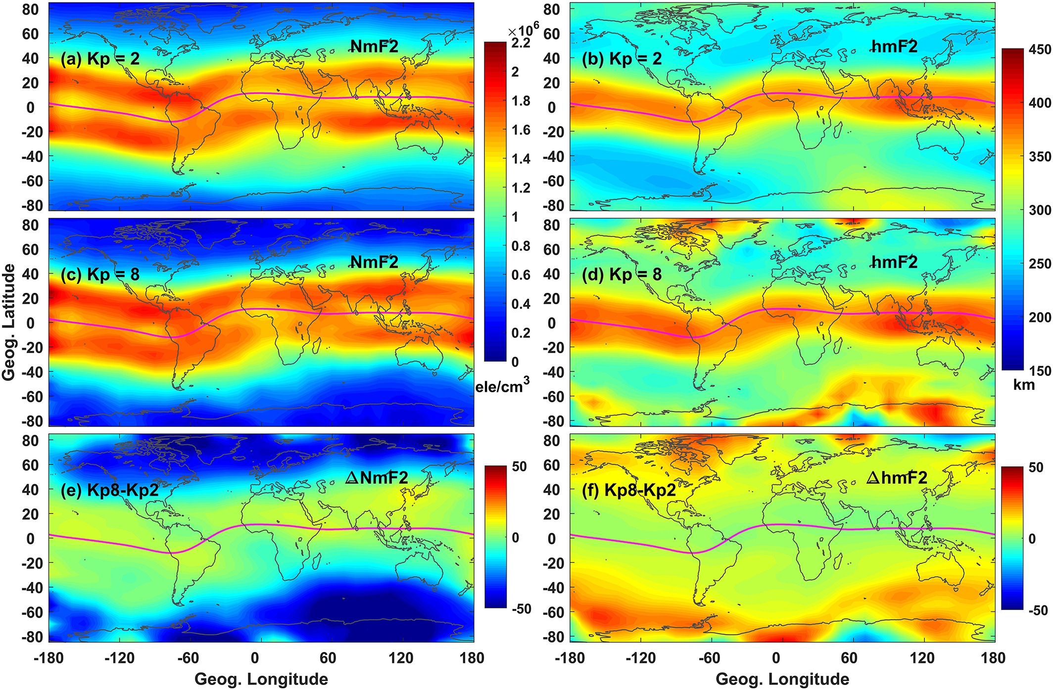
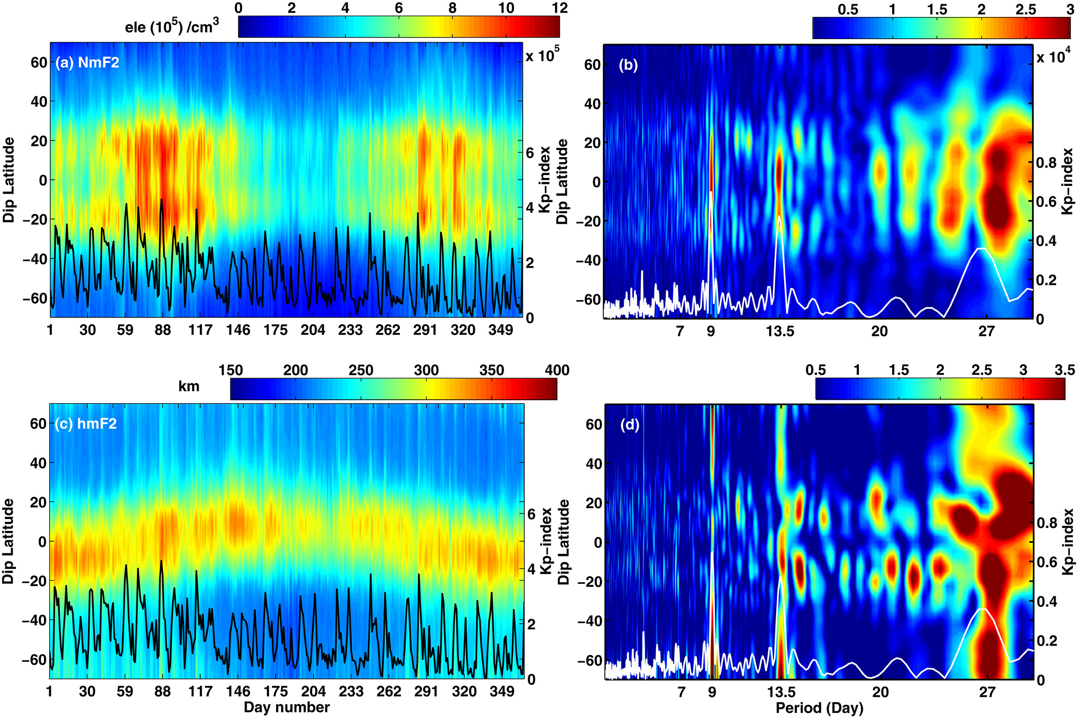
• Reproduced diurnal and seasonal variations of NmF2/hmF2.
• Captured Equatorial Ionization Anomaly (EIA), annual anomaly, Weddell Sea anomaly.
• Improved representation of postsunset hmF2 enhancement in equatorial regions (first reported in later ANNIM-2D upgrades).
• Demonstrated that machine learning can distinguish solar irradiance vs geomagnetic forcing through controlled ANN simulations.

Implications / Applications

• Demonstrated feasibility of data-driven space weather forecasting.
• Formed the foundational prototype for the ANNIM-2D (JGR 2018) and ANNIM-3D models used in later publications.
• Provided a generalizable recipe for physics-informed neural networks in geospace modeling.

Further Reading

• Tulasi Ram et al. (2018), The Improved Two‐Dimensional Artificial Neural Network‐Based Ionospheric Model, JGR Space Physics.
• Gowtam et al. (2019), A New ANN-Based Global Three-Dimensional Ionospheric Model, JGR Space Physics.
• Mitra, A. (2018), MSc Thesis: A Study of Extensive Radio Occultation Data…, PDF.